


-
摘要:
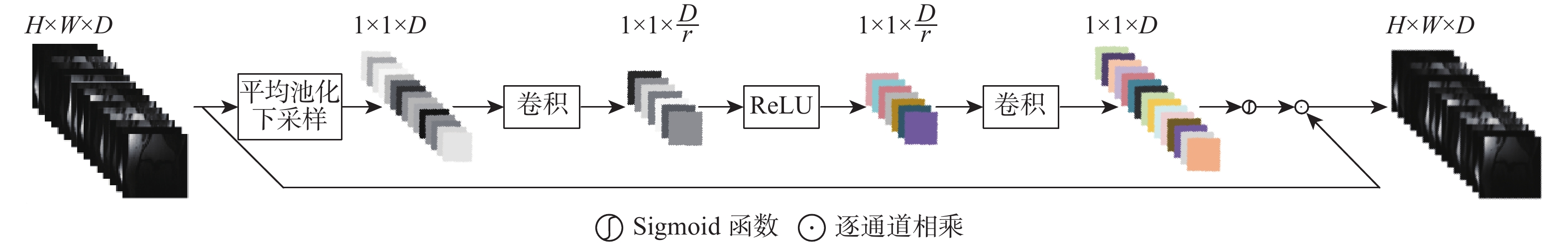
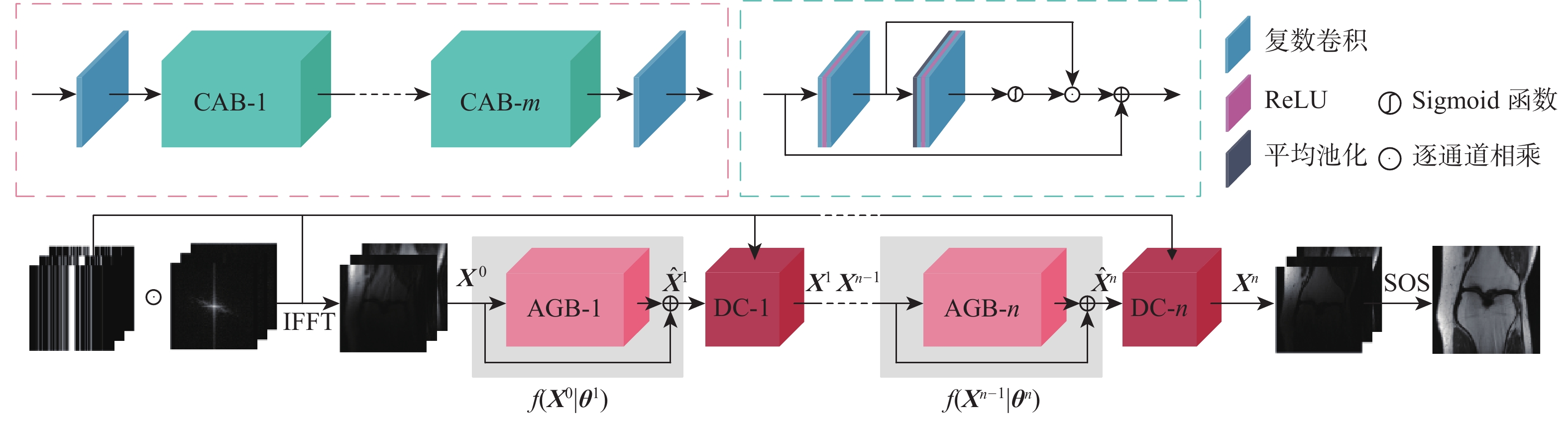
针对并行磁共振成像的重建,提出深度复数注意力网络(DCANet)模型。根据磁共振成像数据的复数性质,该模型使用复数卷积替换常规实数卷积;由于并行磁共振成像的数据中每个线圈获取到的数据有所不同,该模型还使用逐通道的注意力机制来重点关注有效特征较多的通道;该模型使用数据一致性层保留采样过程中的原始数据,最终形成级联网络。使用3个不同的采样模式对2个不同磁共振成像数据序列进行实验,实验结果表明:DCANet模型具有较好的重建效果,能够获得更高的峰值信噪比(PSNR)和结构相似性指数(SSIM),以及更低的高频误差范数(HFEN),其中,PSNR相比磁共振成像级联通道注意力网络(MICCAN)、Deepcomplex、双倍频网络(DONet)这3种模型平均分别提高了4.52 dB、2.30 dB和1.21 dB。
Abstract:for the reconstruction of parallel magnetic resonance imaging, a deep complex attention network (DCANet) model is proposed. A data consistency layer is used to maintain acquired k-space data unchanged, and a cascade network is formed. Additionally, since magnetic resonance images of multiple coils differ, the proposed model also uses a channel-wise attention mechanism to focus on channels with more effective features. All of these techniques are used to replace the conventional method of convolving real and imaginary parts separately in complex convolution. Experiments are conducted on two different magnetic resonance imaging datasets with three different undersampling patterns. According to the experimental findings, the DCANet model performs better during reconstruction and achieves lower high-frequency error norm (HFEN) and greater peak signal-to-noise ratio (PSNR) and structural similarity (SSIM). The DCANet model achieves average PSNR improvements of 4.52 dB, 2.30 dB and 1.21 dB over MRI cascaded channel-wise attention network (MICCAN), Deepcomplex and DONet models, respectively.
-
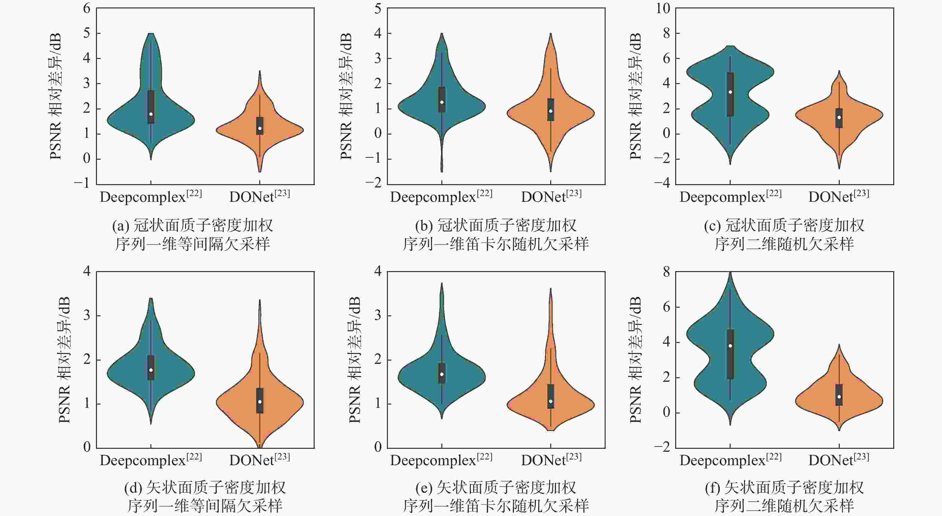

图 4 冠状面质子密度加权序列3倍一维等间隔欠采样重建误差对比
Figure 4. Comparison of reconstruction error maps of coronal plane proton density-weighted sequences with 3-fold 1D uniform undersampled reconstruction
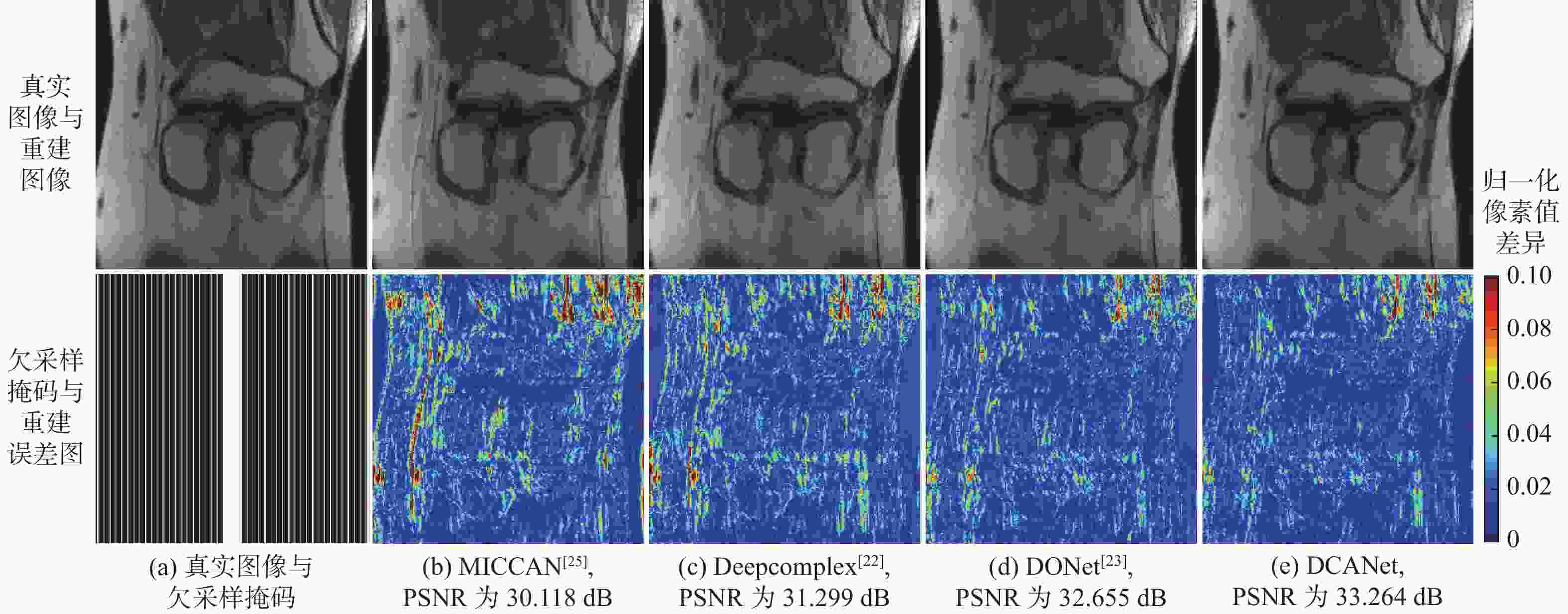
图 5 冠状面质子密度加权序列5倍一维等间隔欠采样重建误差对比
Figure 5. Comparison of reconstruction error maps of coronal plane proton density weighted sequences with 5-fold 1D uniform undersampled reconstruction

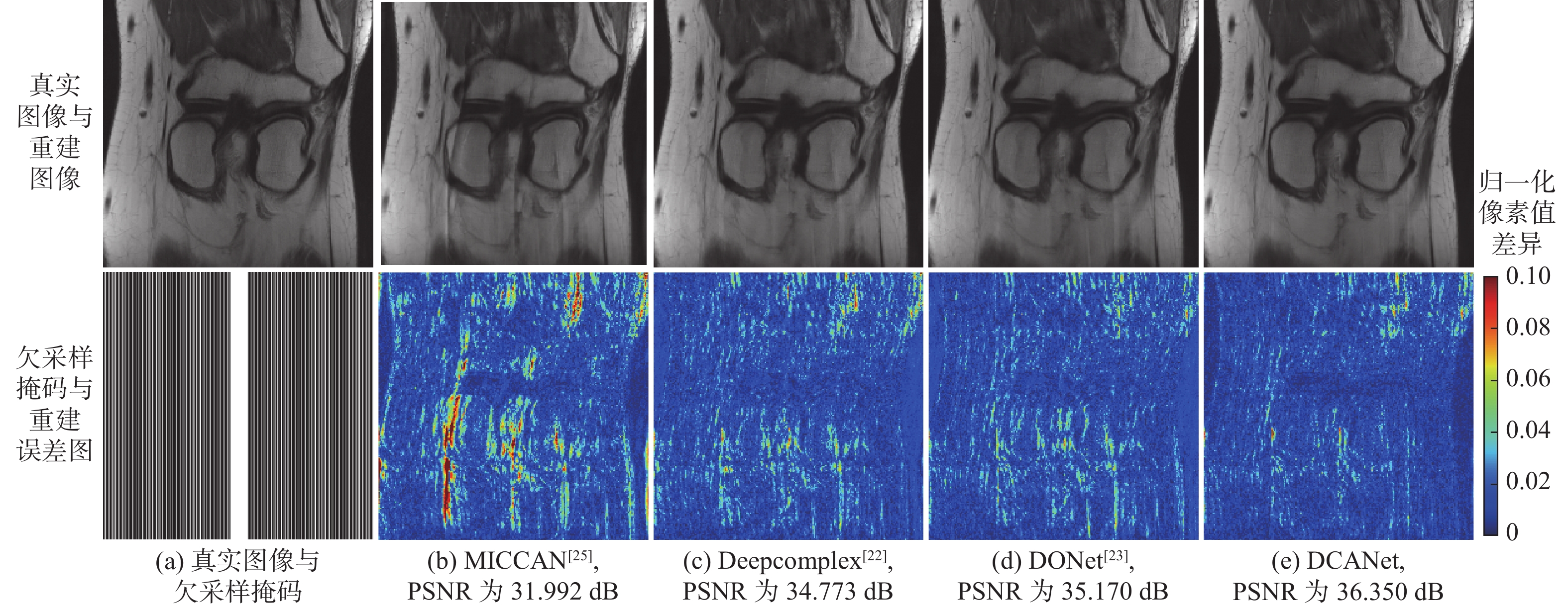
图 6 矢状面质子密度加权序列3倍一维笛卡尔随机欠采样重建误差对比
Figure 6. Comparison of reconstruction error maps of sagittal plane proton density-weighted sequences with 3-fold 1D cartesian random undersampling
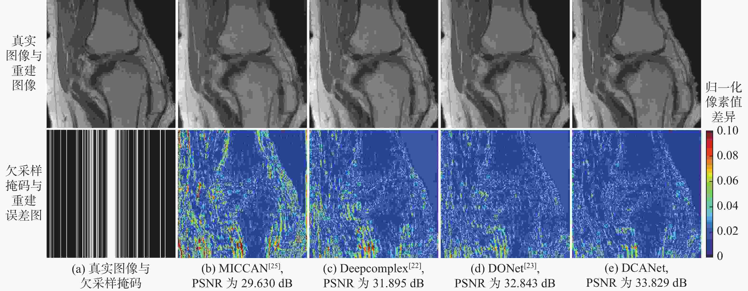
图 7 矢状面质子密度加权序列5倍一维笛卡尔随机欠采样重建误差对比
Figure 7. Comparison of reconstruction error maps of sagittal plane proton density-weighted sequences with 5-fold 1D cartesian random undersampling
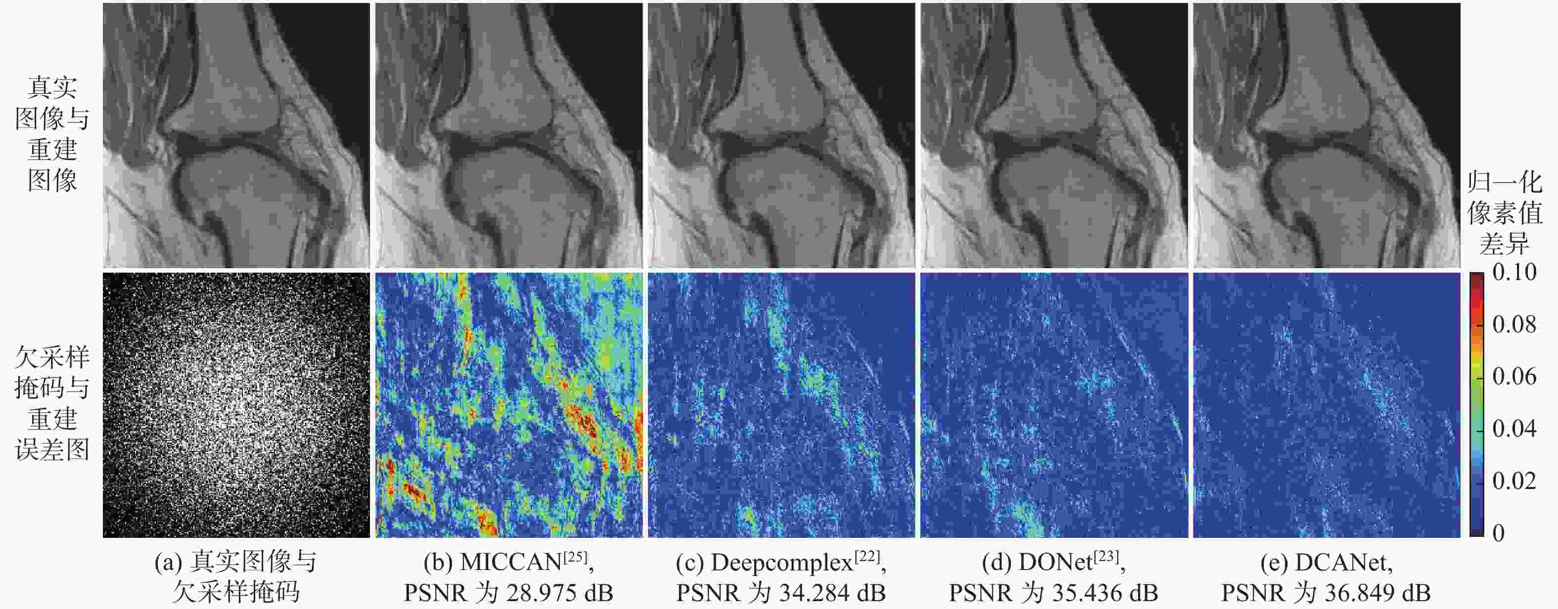
图 8 矢状面质子密度加权序列3倍二维随机欠采样重建误差对比
Figure 8. Comparison of reconstruction error maps of sagittal plane proton density-weighted sequences with 3-fold 2D random undersampling
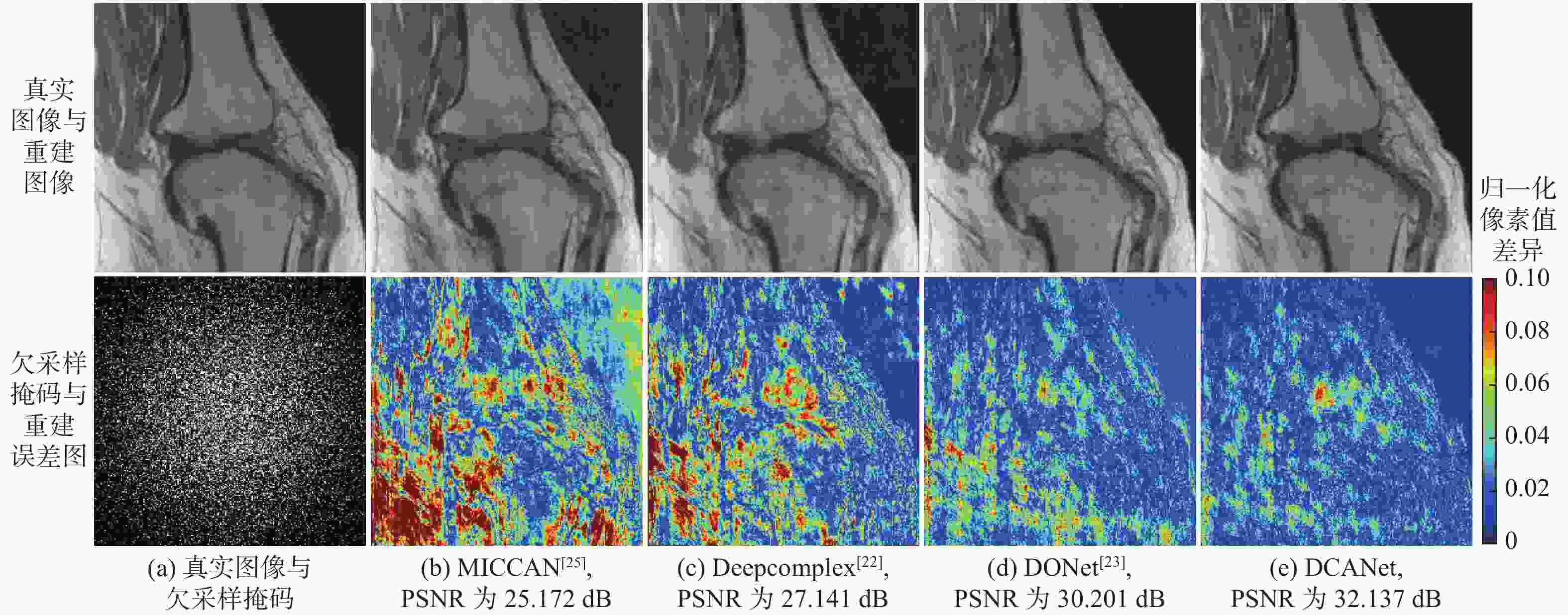
图 9 矢状面质子密度加权序列5倍二维随机欠采样重建误差对比
Figure 9. Comparison of reconstruction error maps of sagittal plane proton density-weighted sequences with 5-fold 2D random undersampling
表 1 DCANet模型参数
Table 1. DCANet model parameters
参数 数值 CAB数量 10 AGB数量 10 Batch Size 1 卷积核大小 3$ \times $3 ${{\boldsymbol{K}}_{{U}{\text{p}}}}$、${{\boldsymbol{K}}_{{\text{Down}}}}$卷积核大小 1×1 ${{\boldsymbol{K}}_{{U}{\text{p}}}}$、${{\boldsymbol{K}}_{{\text{Down}}}}$通道变化率$r$ 8 初始学习率 0.0003 学习率衰减因子 0.7 epoch 300  下载: 导出CSV
表 2 冠状面质子密度加权序列重建效果
Table 2. Reconstruction performance of coronal proton-density weighted sequence
欠采样模式 模型 PSNR/dB SSIM HFEN 3 5 3 5 3 5 一维等间隔欠采样 MICCAN[25] 31.695±0.899 29.973±0.895 0.831±0.016 0.773±0.020 0.385±0.062 0.485±0.058 Deepcomplex[22] 32.708±1.519 29.608±2.111 0.835±0.027 0.754±0.031 0.320±0.085 0.483±0.129 DONet[23] 33.308±1.347 30.693±1.427 0.846±0.025 0.776±0.024 0.303±0.073 0.438±0.107 DCANet 34.786±1.497 31.880±1.398 0.876±0.024 0.812±0.029 0.273±0.069 0.403±0.092 一维笛卡尔随机欠采样 MICCAN[25] 34.515±0.982 32.326±0.946 0.872±0.019 0.818±0.027 0.243±0.046 0.354±0.057 Deepcomplex[22] 35.586±1.385 33.039±1.243 0.880±0.021 0.818±0.029 0.193±0.041 0.299±0.072 DONet[23] 35.799±1.443 33.601±1.254 0.884±0.022 0.828±0.026 0.188±0.040 0.275±0.054 DCANet 36.791±1.298 34.687±1.206 0.899±0.019 0.855±0.028 0.181±0.040 0.266±0.062 二维随机欠采样 MICCAN[25] 30.446±2.190 25.881±2.826 0.876±0.021 0.783±0.034 0.193±0.043 0.322±0.073 Deepcomplex[22] 35.591±2.923 28.795±2.346 0.915±0.025 0.803±0.029 0.122±0.033 0.322±0.049 DONet[23] 36.094±2.560 31.847±2.716 0.920±0.026 0.855±0.031 0.113±0.029 0.206±0.057 DCANet 36.917±2.849 33.596±2.843 0.935±0.017 0.891±0.022 0.103±0.028 0.176±0.048
下载: 导出CSV
表 3 矢状面质子密度加权序列重建效果
Table 3. Reconstruction performance of sagittal proton-density weighted sequence
欠采样掩码 模型 PSNR/dB SSIM HFEN 3 5 3 5 3 5 一维等间隔欠采样 MICCAN[25] 33.710±2.097 29.559±1.726 0.854±0.033 0.731±0.045 0.353±0.051 0.595±0.069 Deepcomplex[22] 35.220±1.868 30.766±1.772 0.870±0.024 0.755±0.037 0.282±0.031 0.502±0.053 DONet[23] 35.744±1.758 31.707±1.603 0.876±0.023 0.773±0.030 0.263±0.028 0.463±0.053 DCANet 37.046±2.069 32.668±1.713 0.900±0.025 0.809±0.034 0.241±0.025 0.426±0.047 一维笛卡尔随机欠采样 MICCAN[25] 34.513±1.862 32.496±1.772 0.864±0.027 0.808±0.035 0.294±0.035 0.404±0.049 Deepcomplex[22] 36.889±1.590 34.342±1.632 0.893±0.019 0.833±0.027 0.194±0.020 0.288±0.029 DONet[23] 37.308±1.541 34.931±1.578 0.896±0.018 0.840±0.026 0.184±0.019 0.267±0.029 DCANet 38.660±1.730 36.073±1.849 0.916±0.020 0.871±0.030 0.168±0.019 0.252±0.031 二维随机欠采样 MICCAN[25] 27.841±3.032 26.252±0.051 0.819±0.057 0.735±0.061 0.267±0.051 0.405±0.067 Deepcomplex[22] 36.025±2.099 29.177±2.295 0.920±0.018 0.802±0.042 0.151±0.018 0.366±0.036 DONet[23] 37.149±1.901 32.905±2.804 0.933±0.014 0.877±0.027 0.130±0.015 0.217±0.031 DCANet 38.166±2.076 34.007±2.209 0.941±0.013 0.894±0.022 0.111±0.013 0.194±0.024
下载: 导出CSV
表 5 数据一致性层对比实验结果
Table 5. Results of data consistency layer contrast experiment
模型 PSNR/dB SSIM HFEN DCANet_NoDC 33.677±1.337 0.857±0.029 0.271±0.052 DCANet 36.791±1.298 0.899±0.019 0.181±0.040
下载: 导出CSV
-
[1] 赵喜平. 磁共振成像[M]. 北京: 科学出版社, 2004: 64-87.ZHAO X P. Magnetic resonance imaging[M]. Beijing: Science Press, 2004: 64-87(in Chinese). [2] DONOHO D L. Compressed sensing[J]. IEEE Transactions on Information Theory, 2006, 52(4): 1289-1306. doi: 10.1109/TIT.2006.871582 [3] LUSTIG M, DONOHO D L, SANTOS J M, et al. Compressed sensing MRI[J]. IEEE Signal Processing Magazine, 2008, 25(2): 72-82. doi: 10.1109/MSP.2007.914728 [4] LAI Z Y, QU X B, LIU Y S, et al. Image reconstruction of compressed sensing MRI using graph-based redundant wavelet transform[J]. Medical Image Analysis, 2016, 27: 93-104. doi: 10.1016/j.media.2015.05.012 [5] KNOLL F, BREDIES K, POCK T, et al. Second order total generalized variation (TGV) for MRI[J]. Magnetic Resonance in Medicine, 2011, 65(2): 480-491. doi: 10.1002/mrm.22595 [6] YANG J F, ZHANG Y, YIN W T. A fast alternating direction method for TVL1-L2 signal reconstruction from partial Fourier data[J]. IEEE Journal of Selected Topics in Signal Processing, 2010, 4(2): 288-297. doi: 10.1109/JSTSP.2010.2042333 [7] PRUESSMANN K P. Encoding and reconstruction in parallel MRI[J]. NMR in Biomedicine, 2006, 19(3): 288-299. doi: 10.1002/nbm.1042 [8] PRUESSMANN K P, WEIGER M, BÖRNERT P, et al. Advances in sensitivity encoding with arbitrary k-space trajectories[J]. Magnetic Resonance in Medicine, 2001, 46(4): 638-651. doi: 10.1002/mrm.1241 [9] PRUESSMANN K P, WEIGER M, SCHEIDEGGER M B, et al. SENSE: Sensitivity encoding for fast MRI[J]. Magnetic Resonance in Medicine, 1999, 42(5): 952-962. doi: 10.1002/(SICI)1522-2594(199911)42:5<952::AID-MRM16>3.0.CO;2-S [10] GRISWOLD M A, JAKOB P M, HEIDEMANN R M, et al. Generalized autocalibrating partially parallel acquisitions (GRAPPA)[J]. Magnetic Resonance in Medicine, 2002, 47(6): 1202-1210. doi: 10.1002/mrm.10171 [11] LUSTIG M, PAULY J M. SPIRiT: Iterative self-consistent parallel imaging reconstruction from arbitrary k-space[J]. Magnetic Resonance in Medicine, 2010, 64(2): 457-471. doi: 10.1002/mrm.22428 [12] UECKER M, LAI P, MURPHY M J, et al. ESPIRiT: An eigenvalue approach to autocalibrating parallel MRI: Where SENSE meets GRAPPA[J]. Magnetic Resonance in Medicine, 2014, 71(3): 990-1001. doi: 10.1002/mrm.24751 [13] LECUN Y, BENGIO Y, HINTON G. Deep learning[J]. Nature, 2015, 521: 436-444. doi: 10.1038/nature14539 [14] RONNEBERGER O, FISCHER P, BROX T. U-net: Convolutional networks for biomedical image segmentation[C]//Proceedings of the European Conference on Computer Vision. Berlin: Springer, 2015: 234-241. [15] DONG C, LOY C C, HE K, et al. Learning a deep convolutional network for image super-resolution[C]//Proceedings of the European Conference on Computer Vision. Berlin: Springer, 2014: 184-199. [16] 施俊, 汪琳琳, 王珊珊, 等. 深度学习在医学影像中的应用综述[J]. 中国图象图形学报. 2020, 25(10): 1953-1981.SHI J, WANG L L, WANG S S, et al. A review of the application of deep learning in medical imaging[J]. Journal of Image and Graphics. 2020, 25(10): 1953-1981(in Chinese). [17] WANG S S, SU Z H, YING L, et al. Accelerating magnetic resonance imaging via deep learning[C]//Proceedings of the IEEE 13th International Symposium on Biomedical Imaging. Piscataway: IEEE Press, 2016: 514-517. [18] SCHLEMPER J, CABALLERO J, HAJNAL J V, et al. A deep cascade of convolutional neural networks for dynamic MR image reconstruction[J]. IEEE Transactions on Medical Imaging, 2018, 37(2): 491-503. doi: 10.1109/TMI.2017.2760978 [19] SRIRAM A, ZBONTAR J, MURRELL T, et al. GrappaNet: Combining parallel imaging with deep learning for multi-coil MRI reconstruction[C]//Proceedings of the IEEE/CVF Conference on Computer Vision and Pattern Recognition. Piscataway: IEEE Press, 2020: 14303-14310. [20] LU T Y, ZHANG X L, HUANG Y H, et al. pFISTA-SENSE-ResNet for parallel MRI reconstruction[J]. Journal of Magnetic Resonance, 2020, 318: 106790. doi: 10.1016/j.jmr.2020.106790 [21] TRABELSI C, BILANIUK O, ZHANG Y, et al. Deep complex networks[EB/OL]. (2017-03-27)[2022-12-14]. http://arxiv.org/abs/1705.09792. [22] WANG S S, CHENG H T, YING L, et al. Deep complexMRI: Exploiting deep residual network for fast parallel MR imaging with complex convolution[J]. Magnetic Resonance Imaging, 2020, 68: 136-147. doi: 10.1016/j.mri.2020.02.002 [23] FENG C M, YANG Z Y, FU H Z, et al. DONet: Dual-octave network for fast MR image reconstruction[C]//Proceedings of the IEEE Transactions on Neural Networks and Learning Systems. Piscataway: IEEE Press, 2021: 1-11. [24] ZHANG Y L, LI K P, LI K, et al. Image super-resolution using very deep residual channel attention networks[C]//Proceedings of the European Conference on Computer Vision. Berlin: Springer, 2018: 294-310. [25] HUANG Q Y, YANG D, WU P X, et al. MRI reconstruction via cascaded channel-wise attention network[C]//Proceedings of the IEEE 16th International Symposium on Biomedical Imaging. Piscataway: IEEE Press, 2019: 1622-1626. [26] HAMMERNIK K, KLATZER T, KOBLER E, et al. Learning a variational network for reconstruction of accelerated MRI data[J]. Magnetic Resonance in Medicine, 2018, 79(6): 3055-3071. doi: 10.1002/mrm.26977 -

 下载:
下载:


 点击查看大图
计量
- 文章访问数: 687
- HTML全文浏览量: 141
- PDF下载量: 26
- 被引次数: 0
